Spreadsheets – Excel

Exercise: New York City’s public employee payroll
Selecting Cells
There are a variety of ways to select cells in an Excel spreadsheet:
To select one cell, click in the cell.
To select one or more rows of cells, click on the row number(s).
To select one or more columns of cells, click on the column letter(s).
To select a group of contiguous cells, click in a corner cell and, with the shift key depressed, drag the cursor horizontally and/or vertically until all of the cells you want selected are outlined.
To select multiple cells that are not contiguous, press and hold the Command key while clicking in the desired cells.
To select every cell in the worksheet, click in the upper right corner of the worksheet to the left of “A.”
To select a row of data, click in the first cell then hit control-shift-right arrow. You can also use the down, left and up arrows.
Jump to the bottom of data with Cmd+Down Arrow, jump back up with Cmd + Up Arrow
To navigate to the four corners of the spreadsheet, click Ctrl period.
Entering Data into Cells
To enter data into a cell, just click in the cell and begin typing. What you type also displays in the Formula Bar. When entering dates, Excel defaults to the current year if the year portion of the date is not entered.
You may edit cell contents from the Formula bar, or from directly inside the cell. To edit from the Formula Bar, select the cell and click inside the Formula Bar. When done typing, either press the Enter key or click inside another cell. To edit directly inside a cell, either double click inside the cell, or select the cell and press the F2 key.
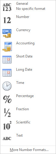
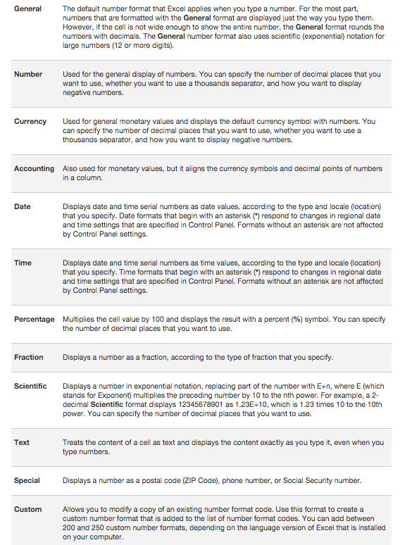
Each cell has a specific format. This format tells Excel how the data inside the cell should be displayed.
Moving and Copying Cells
To move cell contents, right-click in the selected cell and click Cut. To copy cell contents, click Copy. Then right-click in the new location and click Paste. To paste a group of cells, right-click in the cell where the top left cell of the group should be located, and click Paste. Remove the animated border around the original cell by pressing the ESC key, or start typing in a new cell.
Adding and Deleting Rows and Columns
To insert a new row in a spreadsheet, right-click on a row number, and click Insert. To delete a row, right-click on the row number, and click Delete. To insert a new column, right-click on a column letter and click Insert. To delete a column, right-click on the column letter, and click Delete.
Sorting
– No empty rows or columns
– Command A – select all
– Using icons
– Multiple sort
– Sort sheet vs. sort. Decide if you want to sort the entire worksheet or just a cell range. Sort sheet organizes all of the data in your worksheet by one column.
Filtering
– Text, date, numerical
Formulas
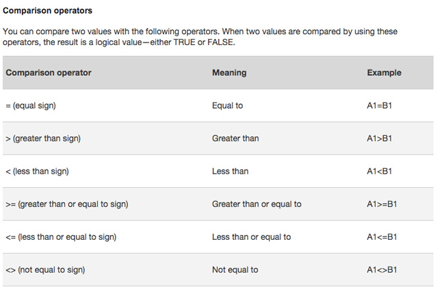
A formula performs calculations or other actions on the data in your worksheet. A formula always starts with an equal sign (=), which can be followed by numbers, math operators (such as a plus or minus sign), and functions, which can really expand the power of a formula.
For example, the following formula multiplies 2 by 3 and then adds 5 to that result to come up with the answer, 11.
=2*3+5
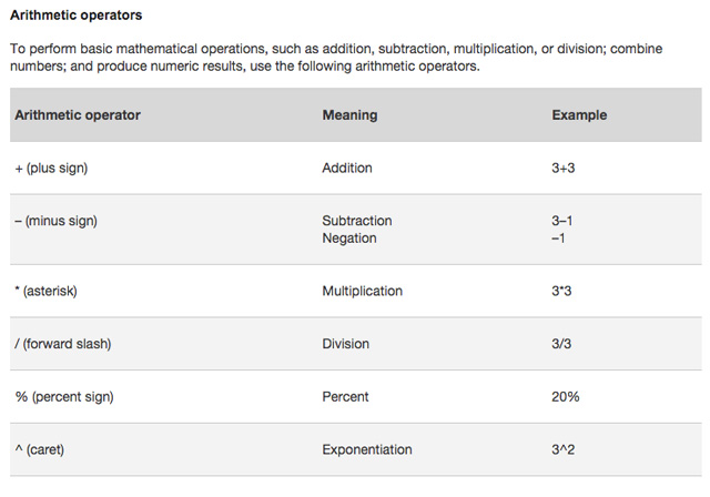
Addition, subtraction, multiplication, division: +, -, *, /
The parts of an Excel formula
A formula can also contain any or all of the following: functions, references, operators, and constants.
Parts of a formula
1. Functions: The PI() function returns the value of pi: 3.142…SUM(A1:A10) returns the sum of those values.
2. References: A2 returns the value in cell A2.
3. Constants: Numbers or text values entered directly into a formula, such as 2.
4. Operators: The ^ (caret) operator raises a number to a power, and the * (asterisk) operator multiplies numbers.
Common Functions
AVERAGE
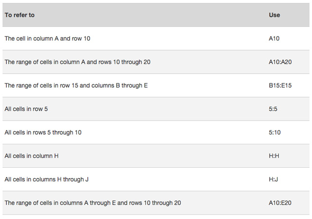
Type =Average(range of cells) and then hit return. Ranges for any function should be enclosed by () and the first and last data value separated by a colon. For example if you want the mean of values in cells A3 to A9 then type =Average(A3:A9).
SUM, MEDIAN, MAX, MIN
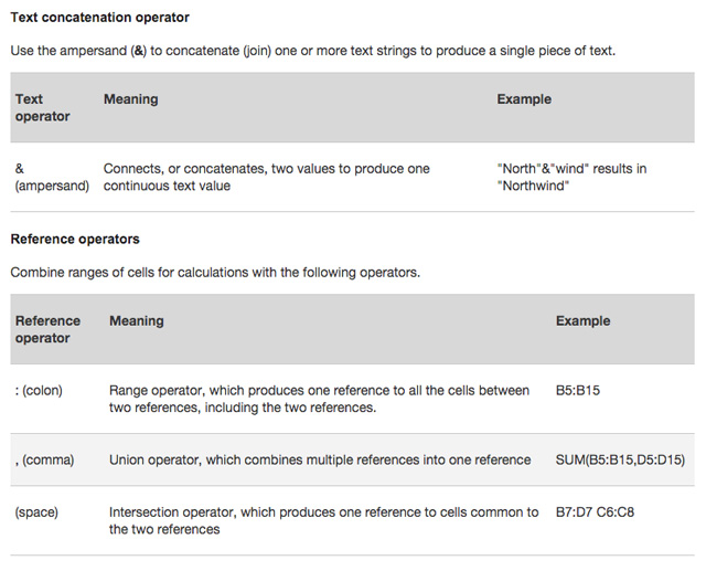
CONCATENATE
Some times the data you find will not have the header in one row and you will need to combine text in one row before using. To do so, use concatenate to create a new header with all of the text elements.
Imagine you have three rows of header information that you need to combine into one.
=CONCATENATE(D1,D2,D3) in cell D4 and hit return. That takes all the text and puts it in one cell.
Next add spaces between words to make the text readable. Include &” “ (a space between the quotes). Change your formula so that it looks like this: =CONCATENATE(D1&” “,D2&” “,D3) to add spaces between the words.
Use of parentheses in Excel formulas
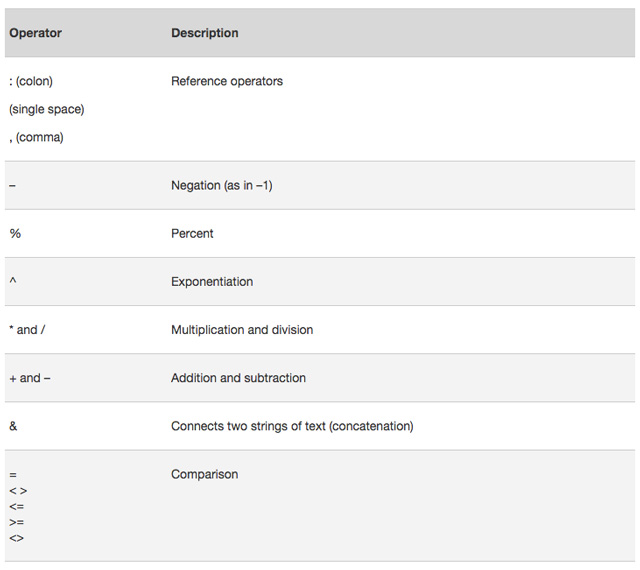
To change the order of evaluation, enclose in parentheses the part of the formula to be calculated first. For example, the following formula produces 11 because Excel performs multiplication before addition. The formula multiplies 2 by 3 and then adds 5 to the result.
=5+2*3
In contrast, if you use parentheses to change the syntax, Excel adds 5 and 2 together and then multiplies the result by 3 to produce 21.
=(5+2)*3
In the following example, the parentheses that enclose the first part of the formula force Excel to calculate B4+25 first and then divide the result by the sum of the values in cells D5, E5, and F5.
=(B4+25)/SUM(D5:F5)
Apply a number format
To distinguish between different types of numbers, add a format, like currency, percentages, or dates.
Select the cells that have numbers you want to format.
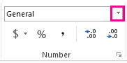
Click Home > Arrow next to General.